Background
In this background page, we explore in more detail the geometric properties of the short-and-sparse deconvolution (SaSD) problem. Typical optimization formulations of SaSD are nonconvex. This nonconvexity can be attributed to the signed shift symmetry of the short-and-sparse model: because of symmetry there are many distinct minimizers. Understanding the geometry of SaSD will enable us to give provable algorithms for certain model problem instances, and, more importantly, to develop better practical algorithms.
Bilinear Lasso and Approximations
Our study centers around the “bilinear Lasso” formulation:
\[ \min_{\mathbf a\in\mathbb S^{p-1},\, \mathbf x\in\mathbb R^{n}} \lambda \lVert \mathbf x\rVert_1 + \tfrac12 \lVert\mathbf a*\mathbf x - \mathbf y\rVert_2^2, \]
which balances sparsity and fidelity to the observed data.
To study its geometry rigorously, we develop an approximation to this objective function, by approximating the loss as
\[ \begin{aligned} & \tfrac12 \lVert\mathbf a*\mathbf x - \mathbf y\rVert_2^2 \\ =\;& \tfrac12 \lVert\mathbf a * \mathbf x \rVert_2^2 - \langle \mathbf a * \mathbf x, \mathbf y \rangle +\tfrac12 \lVert \mathbf y\rVert_2^2 \\ \approx\;& \tfrac12 \lVert\mathbf a \rVert_2^2 + \lVert \mathbf x \rVert_2^2 - \langle \mathbf a * \mathbf x, \mathbf y \rangle +\tfrac12 \lVert \mathbf y\rVert_2^2. \end{aligned}\]
Since both $\lVert\mathbf a\rVert_2^2$ and $\lVert\mathbf y\rVert_2^2$ are constants, the simplified objective becomes
\[ \min_{\mathbf a\in\mathbb S^{p-1},\, \mathbf x\in\mathbb R^{n}} \lambda \lVert \mathbf x\rVert_1 + \tfrac12 \lVert\mathbf x\rVert_2^2 - \langle\mathbf a*\mathbf x,\mathbf y\rangle. \tag{3} \]
This objective still solves the short-and-sparse deconvolution, but requires more stringent signal conditions and larger sample size (longer signal $\mathbf y$); nevertheless, the geometry of this objective represents that of the bilinear-Lasso well and therefore it draws our attention to study it. Specifically, we will investigate the effect of the symmetric solutions of short signal $\mathbf a$ on the objective landscape $\varphi_{\text{ABL}}$, the marginal minimization version of $(3)$, over the sphere $\mathbb S^{p-1}$:
\[ \begin{aligned} &\min_{\mathbf a\in\mathbb S^{p-1} } \varphi_{\text{ABL}}(\mathbf a) \\ :=\;& \min_{\mathbf a\in\mathbb S^{p-1} }\left( \min_{\mathbf x\in\mathbb R^{n}} \lambda \lVert \mathbf x\rVert_1 + \tfrac12 \lVert\mathbf x\rVert_2^2 - \langle\mathbf a*\mathbf x,\mathbf y\rangle\right). \end{aligned}\]
As it turns out, the geometry of this objective will be indeed dictated by the solutions of problem, that is, the shifts of short ground truth $\mathbf a_0$.
From Shifts to Geometry
Shifts of $\mathbf a_0$
From now on, we will assume that the length of the true short signal $\mathbf a_0$ is $p_0$ as that we optimize over a space of dimension $p \geq 3p_0$. Write the shift of $\mathbf a_0$ by $i$ samples as $s_i[\mathbf a_0]$ and put it in the space of dimension $p$, we say
\[ s_i[\mathbf a_0]\,:=\, [\overbrace{0,\ldots,0}^{p+i},\mathbf a_0,\overbrace{0,\ldots,0}^{p-i}] \]
where $i\in \{-p\ldots,p\}$. As we mentioned, these shifts are the solutions to the short-and-sparse deconvolution, which are also the local minimizers of the objective $\varphi_{\text{ABL}}$ and dictate the overall landscape of the objective.
Geometry over subspace of shifts
Specifically, the geometry of $\varphi_{\text{ABL}}$ over the subspace formed by linear combination of a few shifts will exhibit a “symmetric structure”. We will define a subspace spanned by the shifts of $\mathbf a_0$, $s_{\ell_1}[\mathbf a_0],\ldots, s_{\ell_t}[\mathbf a_0]$, as:
\[ \mathcal S_{\{\ell_1,\ldots,\ell_t\}} \,:=\, \mathrm{span}\{s_{\ell_1}[\mathbf a_0],\ldots, s_{\ell_t}[\mathbf a_0]\}. \]
As it turns out, these symmetric structure of landscape for $\varphi_{\text{ABL}}$ over $ \mathcal S_{\{\ell_1,\ldots,\ell_t\}}\cap \mathbb S^{p-1}$ will enable efficient methods to find the ground truth when several conditions on the ground truth signals $(\mathbf a_0,\mathbf x_0)$ are satisfied.
We demonstrate three pictorial examples for the $\varphi_{\text{ABL}}$ landscape over sphere near the subspace that is spanned by one, two, and three shifts, as follows:
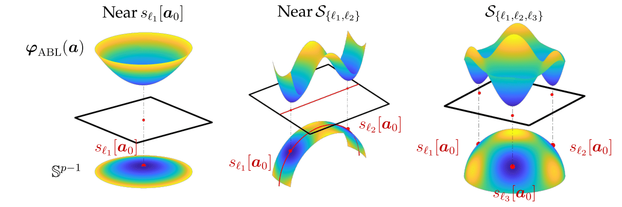
Firstly, the figure on the left shows that the landscape of $\varphi_{\text{ABL}}$ is strongly convex near the shift $s_{\ell_1}[\mathbf a_0]$, and, not-surprisingly, its unique local minimizer is also close to that exact shift. Though this local geometry is certainly ideal for the minimization algorithm to solving the deconvolution problem, this region is very small compared to overall space the sphere $\mathbb S^{p-1}$, meaning that it can be difficult (computationally inefficient) to locate these regions without additional understanding of geometric landscape for $\varphi_{\text{ABL}}$.
Secondly, the figure on the middle shows $\varphi_{\text{ABL}}$ landscape near the subspace $\mathcal S_{\{\ell_1,\ell_2\}}$ spanned by two shifts $s_{\ell_1}[\mathbf a_0], s_{\ell_2}[\mathbf a_0]$ exhibits a symmetric structure. The landscape is constituted by two convex region near either $s_{\ell_1}[\mathbf a_0]$ and $s_{\ell_2}[\mathbf a_0]$; in between the two shifts, the negative curvature of $\varphi_{\text{ABL}}$ breaks this symmetric structure; and away from this subspace, the function values $\varphi_{\text{ABL}}(\mathbf a)$ are growing. Though this geometry is nonconvex, it is expected that a minimization algorithm that starts within this region solves the deconvolution problem, because of two reasons: (1) the minimizing procedure is very unlikely to be stuck in between the symmetric structure—the saddle point has zero measure and has large negative curvature directions pointing at either solutions, and (2) the minimization algorithm will be trapped within this region near subspace, since the function value away from this subspace always grows.
Lastly, the symmetric structure for $\varphi_{\text{ABL}}$ can be extended to higher dimensional subspaces, as we show in the figure on the right, which demonstrates the landscape over span of three shifts $s_{\ell_1}[\mathbf a_0], s_{\ell_2}[\mathbf a_0], s_{\ell_3}[\mathbf a_0]$. Noticeably, all local minimizers are near shifts, and in between all three shifts (the peak point right in the middle), all curvatures with directions inside this subspace are negative; meanwhile, we can also see the substructure formed by any pair of two shifts exhibits similar symmetric structure as in the second figure. Therefore, minimization starts within this subspace can also successfully find the shifts; and more importantly, this geometry structure can be extended to even higher dimensional subspace (much higher then three), and to any subspaces formed by different combinations of shifts.
Finally, we want to list these key findings base on the investigation of this geometry over shifts subspace:
-
Minimizer: Within the subspace, all local minimizers are close to one of the shifts, and all these local regions have symmetric structure.
-
Negative Curvature: Within the subspace, and in between the shifts, the negative curvature of $\varphi_{\text{ABL}}$ will breaks the symmetric structure, meaning that the minimizing algorithm will not stuck in between and will eventually find one of the good local minimizer.
-
Positive Curvature: Away from the subspace, the function value of $\varphi_{\text{ABL}}$ will be growing, meaning that the minimizing algorithm will stay trapped near the subspace over iterates.
Geometry over union of subspaces
The benign geometry of $\varphi_{\text{ABL}}$ for the minimization algorithm to solve the short-and-sparse deconvolution holds not just near a single subspace, but near any subspace formed by span of any different combination of shifts:
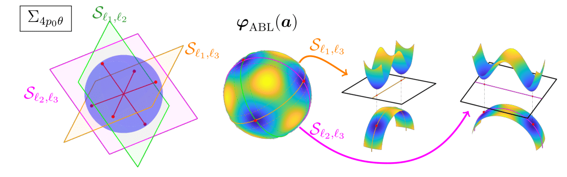
We provide a pictorial example once again, as it shows the geometry of $\varphi_{\text{ABL}}$ over the sphere $\mathbb S^{p-1}$ exhibits similar symmetric structure for every pair of different shifts $(s_{\ell_1}[\mathbf a_0], s_{\ell_2}[\mathbf a_0])$, $(s_{\ell_2}[\mathbf a_0], s_{\ell_3}[\mathbf a_0])$ and $(s_{\ell_3}[\mathbf a_0], s_{\ell_1}[\mathbf a_0])$, in which all the local minimizers of $\varphi_{\text{ABL}}$ over this union of subspace are close to shifts that span the subspace. Similar geometric property holds for union of shifts subspaces of much higher dimension. In theory, depending on $p_0$ the length of $\mathbf a_0$ and $\theta$ the sparsity rate of $\mathbf x_0$, this preferable geometry holds for union of subspaces spanned any combination of $4p_0\theta$ shifts.
When is SaSD Solvable?
Short-and-sparse deconvolution is impossible in general, but it can be solved efficiently, whenever the following conditions are satisfied:
-
Short: $\mathbf a_0$ is enough short compares to the observed signal.
-
Incoherence: all signed shifts of $\mathbf a_0$ are not close to each other in $\ell^2$ distance.
-
Sparse: The density of the support for $\mathbf x_0$ is sufficiently sparse, and somewhat irregular.
There is a catch here, if we push these conditions to extreme, say if the pattern is so short and the map is sparse enough that most of the patterns being non overlapping, then short-and-sparse deconvolution problem becomes trivial—-which simply boils down to looking for the isolated short signal as the ground truth $\mathbf a_0$. This extreme case does not apply to most of the practical scenarios, and a well designed algorithm should be able to solve short-and-sparse deconvolution even under other more complicated, non-trivial cases.
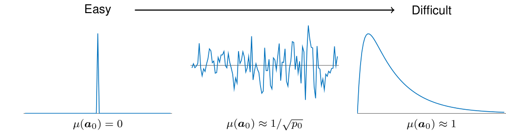
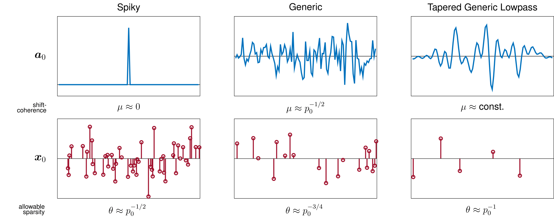
Shift coherence of $\mathbf a_0$
Short-and-sparse deconvolution becomes an easier problem if the short $\mathbf a_0$ is more shift-incoherent. The coherence $\mu(\mathbf a_0)\in[0,1]$ is simply defined as the largest absolute inner-product between all different shift pairs, namely
\[ \mu(\mathbf a_0) \,:=\, \max_{i\neq j}\; \lvert\langle s_i[\mathbf a_0], s_j[\mathbf a_0] \rangle\rvert. \]
$\mu(\mathbf a_0)$ characterizes the difference between the solutions of short-and-sparse deconvolution: if the coherence is larger $\mu(\mathbf a_0)\nearrow 1$, then there are two shifts being closer on the sphere, which will be harder for the algorithm to distinguish whether the shift of $\mathbf a_0$ is fitting to solve the problem. Geometrically speaking, the closer these shifts are, the easier a bad local minimizer may be created in between the shift, and the algorithm could wrongly report this minimizer, the linear combination of shifts, as the solution.
Generally speaking, if the spectrum of the short $\mathbf a_0$ is biased ($\mathbf a_0$ is lowpass, highpass, etc.), then the coherence of $\mathbf a_0$ tends to become larger, and vice versa.
Sparsity of $\mathbf x_0$
We characterize the sparsity of $\mathbf x_0$ by assuming it to be a random vector whose entries are subordinate to Bernoulli-Gaussian distribution with support activation rate $\theta$.
\[ \mathbf x_0 \sim_{\text{i.i.d.}}\text{BG}(\theta) \]
Concretely, the random vector $\mathbf x_0$ can be written as $\mathbf x_0 = \mathbf g \circ \mathbf \omega$ where $\mathbf g$ is Gaussian vector $\mathbf g \sim_{\text{i.i.d.}} \mathcal N(0,1) \in\mathbb R^n$ and $\mathbf \omega$ is Bernoulli vector $\mathbf\omega\sim_{\text{i.i.d.}}\text{Ber}(\theta) \in\mathbb R^n $.
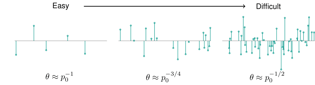
As expected, when the sparsity $\theta$ is higher, the short-and-sparse deconvolution problem becomes harder, and vice versa. Notice, that if the sparsity rate $\theta$ is lesser then $1/p_0$, there will have many isolated $\mathbf a_0$ in the observation signal $\mathbf y$ that can be found via simply algorithm, which makes the short-and-sparse deconvolution a trivial problem. The algorithm we are studying works under more complicating signal condition, namely when $\theta \geq 1/p_0$.
Sparsity-coherence tradeoff
We can further articulate these conditions for solving short-and-sparse deconvolution through “sparsity-coherence tradeoff”. That is, the deconvolution problem becomes easier to solve when either the short $\mathbf a_0$ has low coherence $\mu(\mathbf a_0) \searrow 0$ or the sparsity of $\mathbf x_0$ is lower $\theta \searrow 1/p_0$. If the short $\mathbf a_0$ has low shift-coherence, then the sparsity of $\mathbf x_0$ is allowable to larger, and if $\mathbf a_0$ turns out to be smoother and low-pass, then the allowable of $\mathbf x_0$ has to be lower.
From Geometry to Algorithm
The understanding of how the geometry of $\varphi_{\text{ABL}}$ is shaped by the shifts of $\mathbf a_0$ suggests it is possible to design an algorithm that guarantees solving short-and-sparse deconvolution. The algorithm is straightforward. It starts near one of the shift subspaces, and stays near the subspace through the course of minimization.
Initialization in union of subspaces
Let us consider a case where the observation of noiseless $\mathbf y$ consists of isolated, non-overlapping $\mathbf a_0$. In this trivial case, solving the deconvolution problem becomes finding the isolated copy of the short signal $\mathbf a_0$, which can be done via locating the shortest continuous segment of $\mathbf y$, simple as it can possibly be. This algorithm, though, is unrealistic in even slightly more general cases, when $\mathbf y$ contains noise or $\mathbf x_0$ has higher sparsity.
Nevertheless, we can still adopt this idea under realistic scenarios when $\mathbf y$ contains noise and overlapping $\mathbf a_0$ by seeing that, due to the sparsity of $\mathbf x_0$, a chunk of data $[\mathbf y_1,\ldots,\mathbf y_p]$ will contain only a few shifts of $\mathbf a_0$. This observation implies that a chunk of $\mathbf y$ will be closer to the set of the shifts, and will be close to the shift subspace where $\varphi_{\text{ABL}}$ has nice geometry.
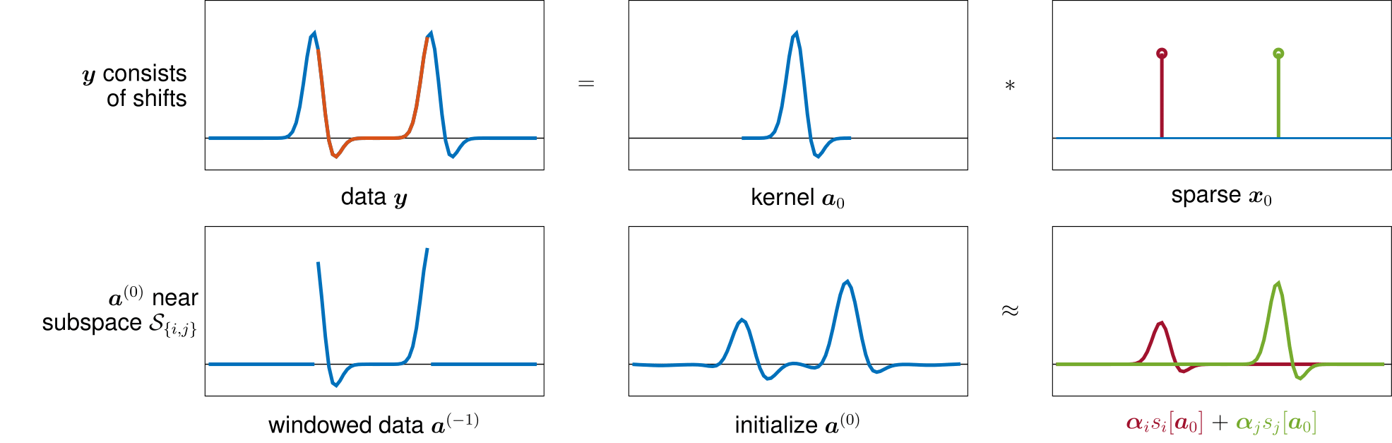
The figure shows an example where the chunk of the data $\mathbf y$ contains a few truncated shift of $\mathbf a_0$, and with simple modification (taking gradient) we can easily obtain a initial vector that stays in the subspace spanned by these shifts. When the sparsity of $\mathbf x_0$ is $\theta$, then in expectation, the number of participating shift in this initialization scheme is roughly about $3p_0\theta$. Since, it is known that $\varphi_{\text{ABL}}$ has nice geometry over subspace with dimension up to $4p_0\theta$, it is expected that minimization starting with the appointed $\mathbf a^{(0)}$ solves the deconvolution problem.
As it turns out, this initialization $\mathbf a^{(0)}$ using a chunk of data $\mathbf y$, can be also applied to the practical problems using bilinear-lasso.
Minimization within the subspace
Finally, knowing that the function value of $\varphi_{\text{ABL}}$ is growing away from the subspace, implies the small stepping gradient descent method on this objective will not leave the subspace, and will eventually converge to a local minimizer within, which are exactly the solution, shifts of $\mathbf a_0$.
To adopt this phenomenon in practice while solving bilinear-lasso for deconvolution, since the studied objective $\varphi_{\text{ABL}}$ is the marginal minimization over $\mathbf x$ of the Lasso-like objective, it is advised the initialization $\mathbf x^{(0)}$ should also be the minimizer of the objective with assigned $\mathbf a^{(0)}$, then alternation minimization of both $\mathbf a$ and $\mathbf x$ would well approximate the gradient descent procedure of minimizing $\varphi_{\text{ABL}}$ within the subspace, hence the correct solution can be attained.