Short-and-Sparse Deconvolution
—finding repeated patterns in signals
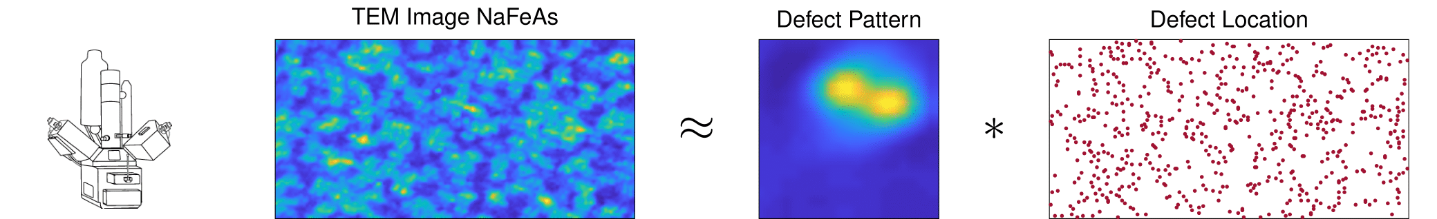
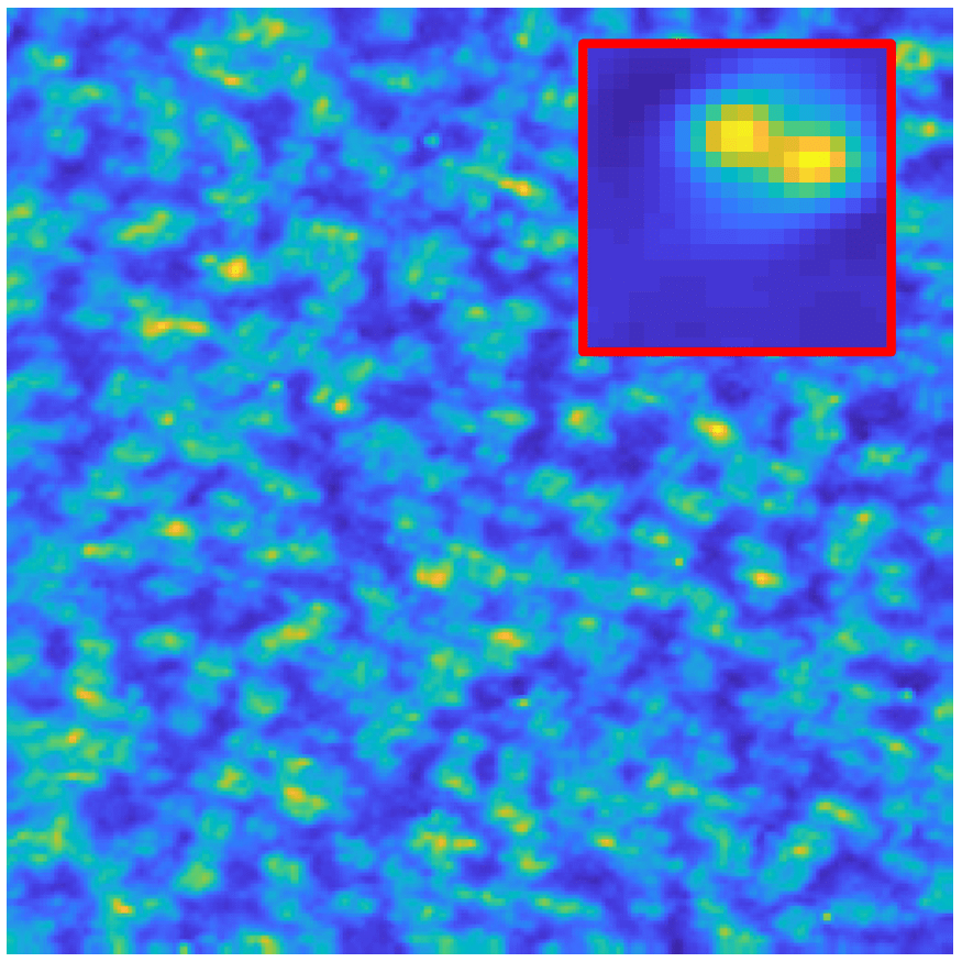 Repeating defect signature of an STM image for superconductor NaFeAs
Many signals and datasets contain one or more basic, repeated motifs. Data of the nature can be modeled as the convolution between a short signal (the motif) and a sparse signal that indicates where in the observed sample the motif occurs. In many applications, neither the motif, nor its locations are known ahead of time, and the goal is to determine both from only the observed data.
We call this problem short-and-sparse deconvolution.
Examples
Signals with short-and-sparse structure arise naturally in many applications. We give several examples below:
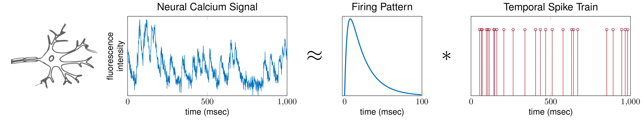
Neural Spike Sorting
Neurons communicate with each other using electric pulses. These pulses can be modeled as the convolution of a (short) neuron firing pattern, and a (sparse) spike train which indicates when the neuron has fired.
Electron Microscopy
In a periodic crystalline structure, the positions of atoms or molecules occur on repeating fixed distances. However, the arrangement in most crystalline materials is not perfect, where the regular patterns are interrupted by defects / vacancies / impurities [4]. Characterization of these atomic defects including the pattern (the short event signal) and the defect locations (the sparse map) affects the bulk electronic and mechanical properties for the materials such as semiconductor, superconductor, etc.
Natural image deblurring
Image deblurring is a classical problem in natural image processing, where the goal is to remove the blurring due to defocus or camera motion. In this scenario, the observed image can be modeled as the convolution of a short blur kernel (which models defocus and sensor motion) with a sharp natural image. While natural images are not sparse, their gradients are typically sparse or compressible, reflecting the fact that natural images typically have relatively few sharp edges [6]. The gradient of the observed image can therefore be modeled as the convolution of a short blur kernel and a sparse signal (the true gradient).

Algorithm Overview
Short-and-sparse deconvolution can be solved via simple, intuitive algorithms. Because variants of short-and-sparse deconvolution arise in a number of applications, many algorithms have been proposed for this problem, and tailored to suit the specific properties of applications.
Here, we describe one general purpose algorithm for short-and-sparse deconvolution, which in some situations recovers the correct short and sparse components, up to a scale and shift symmetry that is intrinsic to the problem.
Symmetric Solutions
The short and sparse model asserts that the observation $\mathbf y$ can be written as a convolution of a short signal $\mathbf a_0 \in\mathbb R^p$ and a sparse signal $ \mathbf x_0\in\mathbb R^n$ $(p\ll n)$: \[\mathbf y \approx \mathbf a_0*\mathbf x_0. \tag{1} \]
This model exhibits a basic signed shift symmetry:
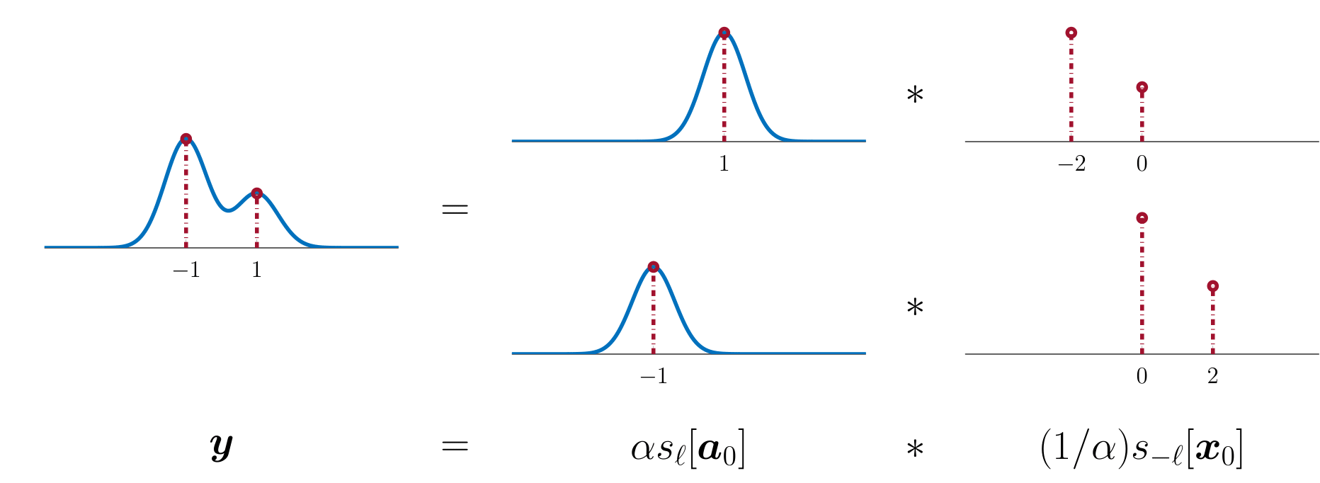
Because of this ambiguity, it is only possible to recover the generating pair $(\mathbf a_0, \mathbf x_0)$ up to scale and shift.
Formulation
To find a shifted and scaled version of $\mathbf a_0\in\mathbb R^p$ and $\mathbf x_0\in\mathbb R^n$, our algorithm optimizes two variables, the short pattern $\mathbf a\in\mathbb R^{3p}$ and the sparsity map $\mathbf x\in\mathbb R^{n+2p}$. A natural approach is to minimize an objective that balances (i) the sparsity of $\mathbf x$ with (ii) the fidelity of $\mathbf a * \mathbf x$ to the observed data $\mathbf y$:
\[ \min_{\mathbf a\in\mathbb S^{3p-1},\, \mathbf x\in\mathbb R^{n+2p}} \overbrace{\lambda \lVert\mathbf x\rVert_1}^{\text{sparsity}} + \overbrace{\tfrac12 \lVert\mathbf a*\mathbf x - \mathbf y\rVert_2^2}^{\text{data fidelity}}. \tag{2} \]
Our approach to this problem is fairly straightforward. There are several details that are helpful for coping with the symmetry structure of the problem:
-
Sphere: We constrain the short variable $\mathbf a$ to have unit $\ell^2$ norm: $\lVert \mathbf a\rVert_2=1$.
-
Zero Padding: The algorithm optimizes the variables $\mathbf a,\mathbf x$ on a higher dimensional space, to accommodate all possible shifts $(\mathbf a_0, \mathbf x_0)$ as good solutions. If the ground truth $\mathbf a_0$ has length $p$, then it is advised to optimize $\mathbf a$ of length $p+2p$, and similarly for $\mathbf x$ of length $n+2p$. Accordingly, the corresponding observation signal $\mathbf y$ should be zero padded on two sides depending on the assumed length of $\mathbf a_0$ during optimization.
Minimizing Algorithm
The optimization problem $(2)$ is a nonconvex. The landscape of the objective is shaped by the symmetries of the problem—shifts of $(\mathbf a_0, \mathbf x_0)$. More importantly, all of the local minimizers of the landscape within some certain region are exactly the shifts, meaning that if we set up the algorithm correctly then the short-and-sparse deconvolution can be solved via minimizing $(2)$.
-
Initialization: Knowing that the solutions are the shifts of $\mathbf a_0$ and $\mathbf x_0$ suggests it would be better starts the minimization with initializer $(\mathbf a^{(0)}, \mathbf x^{(0)})$ closer to the set of shifts. Thus, it is advised to set the $\mathbf a^{(0)}$ as a normalized chunk of data $\mathbf y$ (which indeed will be closer to the solutions compares to, say, a random vector), and the $\mathbf x^{(0)}$ as the minimizer of $(2)$ with fixed $\mathbf a = \mathbf a^{(0)}$
-
$\mathbf a^{(0)} = \frac{[ \overbrace{0,\ldots, 0}^p, \mathbf y_1,\cdots \mathbf y_{p} , \overbrace{0,\ldots, 0}^p]}{ \lVert[\mathbf y_1,\cdots ,\mathbf y_p]\rVert_2}$
-
$\mathbf x^{(0)} = \mathrm{argmin}_{\mathbf x} \,\lambda \lVert x\rVert_1 + \tfrac12\lVert \mathbf a^{(0)}*\mathbf x - \mathbf y \rVert_2^2 $
-
-
Minimization: Starting from the initializer, performing conventional alternating gradient descent on both variables $\mathbf a$ and $\mathbf x$ suffices to solve the problem. Here, the notion of gradient on $\mathbf a$ is Riemmanian, which is nothing special but the conventional gradient defined over spherical domain. Also, the penalty variable in $(2)$, $\lambda$, can be set according to the sparsity level $ \theta$ of the true map $\mathbf x_0$, such that $\lambda \lessapprox 1/\sqrt{p\theta}$.
Code Package
A Matlab solver for short-and-sparse deconvolution can be downloaded from the following github link:
https://github.com/deconvlab/sas-deconv
To exercise the test code, please execute the following code in Matlab console:
$ deconv_example
References
-
For detailed explanation, please refer to the background page.
-
The above exposition is based on the paper “Geometry and Symmetry in Short-and-Sparse Deconvolution” [Short Version] [Long Version]. Please refer to the papers page for additional references and resources.
[1]. Hubel, David H., and Torsten N. Wiesel. “Receptive fields of single neurones in the cat’s striate cortex.” The Journal of physiology 148.3 (1959): 574-591.
[2]. Gerstner, Wulfram, et al. “Neural codes: firing rates and beyond.” Proceedings of the National Academy of Sciences 94.24 (1997): 12740-12741.
[3]. Stosiek, Christoph, et al. “In vivo two-photon calcium imaging of neuronal networks.” Proceedings of the National Academy of Sciences 100.12 (2003): 7319-7324.
[4]. Mura, Toshio. Micromechanics of defects in solids. Springer Science & Business Media, 2013.
[5]. Rosenthal, Ethan P., et al. “Visualization of electron nematicity and unidirectional antiferroic fluctuations at high temperatures in NaFeAs.” Nature physics 10.3 (2014): 225.
[6]. Levin, Anat, et al. “Image and depth from a conventional camera with a coded aperture.” ACM transactions on graphics 26.3 (2007): 70.